Canonical Correlation Analysis Non Continuous Variables
Canonical correlation analysis is used to identify and measure the associations among two sets of variables. Canonical correlation is appropriate in the same situations where multiple regression would be, but where are there are multiple intercorrelated outcome variables. Canonical correlation analysis determines a set of canonical variates, orthogonal linear combinations of the variables within each set that best explain the variability both within and between sets.
This page uses the following packages. Make sure that you can load them before trying to run the examples on this page. If you do not have a package installed, run: install.packages("packagename"), or if you see the version is out of date, run: update.packages().
require(ggplot2) require(GGally) require(CCA)
Version info: Code for this page was tested in R Under development (unstable) (2012-11-16 r61126) On: 2012-12-15 With: CCP 1.1; CCA 1.2; fields 6.7; spam 0.29-2; fda 2.3.2; RCurl 1.95-3; bitops 1.0-5; Matrix 1.0-10; lattice 0.20-10; zoo 1.7-9; GGally 0.4.2; reshape 0.8.4; plyr 1.8; ggplot2 0.9.3; knitr 0.9
Please Note: The purpose of this page is to show how to use various data analysis commands. It does not cover all aspects of the research process which researchers are expected to do. In particular, it does not cover data cleaning and checking, verification of assumptions, model diagnostics and potential follow-up analyses.
Examples of canonical correlation analysis
Example 1. A researcher has collected data on three psychological variables, four academic variables (standardized test scores) and gender for 600 college freshman. She is interested in how the set of psychological variables relates to the academic variables and gender. In particular, the researcher is interested in how many dimensions (canonical variables) are necessary to understand the association between the two sets of variables.
Example 2. A researcher is interested in exploring associations among factors from two multidimensional personality tests, the MMPI and the NEO. She is interested in what dimensions are common between the tests and how much variance is shared between them. She is specifically interested in finding whether the neuroticism dimension from the NEO can account for a substantial amount of shared variance between the two tests.
Description of the data
For our analysis example, we are going to expand example 1 about investigating the associations between psychological measures and academic achievement measures.
We have a data file, mmreg.dta, with 600 observations on eight variables. The psychological variables are locus_of_control, self_concept and motivation. The academic variables are standardized tests in reading (read), writing (write), math (math) and science (science). Additionally, the variable female is a zero-one indicator variable with the one indicating a female student.
mm <- read.csv("https://stats.idre.ucla.edu/stat/data/mmreg.csv") colnames(mm) <- c("Control", "Concept", "Motivation", "Read", "Write", "Math", "Science", "Sex") summary(mm)
## Control Concept Motivation Read ## Min. :-2.2300 Min. :-2.6200 Min. :0.000 Min. :28.3 ## 1st Qu.:-0.3725 1st Qu.:-0.3000 1st Qu.:0.330 1st Qu.:44.2 ## Median : 0.2100 Median : 0.0300 Median :0.670 Median :52.1 ## Mean : 0.0965 Mean : 0.0049 Mean :0.661 Mean :51.9 ## 3rd Qu.: 0.5100 3rd Qu.: 0.4400 3rd Qu.:1.000 3rd Qu.:60.1 ## Max. : 1.3600 Max. : 1.1900 Max. :1.000 Max. :76.0 ## Write Math Science Sex ## Min. :25.5 Min. :31.8 Min. :26.0 Min. :0.000 ## 1st Qu.:44.3 1st Qu.:44.5 1st Qu.:44.4 1st Qu.:0.000 ## Median :54.1 Median :51.3 Median :52.6 Median :1.000 ## Mean :52.4 Mean :51.9 Mean :51.8 Mean :0.545 ## 3rd Qu.:59.9 3rd Qu.:58.4 3rd Qu.:58.6 3rd Qu.:1.000 ## Max. :67.1 Max. :75.5 Max. :74.2 Max. :1.000
Analysis methods you might consider
Below is a list of some analysis methods you may have encountered. Some of the methods listed are quite reasonable while others have either fallen out of favor or have limitations.
- Canonical correlation analysis, the focus of this page.
- Separate OLS Regressions – You could analyze these data using separate OLS regression analyses for each variable in one set. The OLS regressions will not produce multivariate results and does not report information concerning dimensionality.
- Multivariate multiple regression is a reasonable option if you have no interest in dimensionality.
Canonical correlation analysis
Below we use the canon command to conduct a canonical correlation analysis. It requires two sets of variables enclosed with a pair of parentheses. We specify our psychological variables as the first set of variables and our academic variables plus gender as the second set. For convenience, the variables in the first set are called "u" variables and the variables in the second set are called "v" variables.
Let's look at the data.
psych <- mm[, 1:3] acad <- mm[, 4:8] ggpairs(psych) 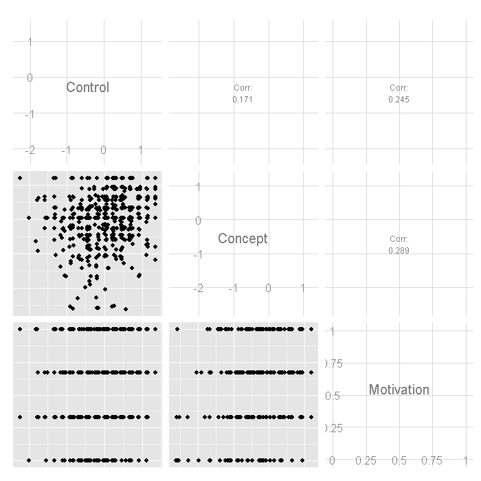
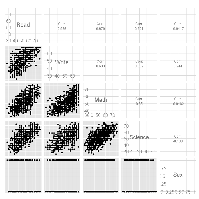
For more information about GGally including packages such as ggduo() you can look here. Next, we'll look at the correlations within and between the two sets of variables using the matcor function from the CCA package.
## $Xcor ## Control Concept Motivation ## Control 1.0000 0.1712 0.2451 ## Concept 0.1712 1.0000 0.2886 ## Motivation 0.2451 0.2886 1.0000 ## ## $Ycor ## Read Write Math Science Sex ## Read 1.00000 0.6286 0.67928 0.6907 -0.04174 ## Write 0.62859 1.0000 0.63267 0.5691 0.24433 ## Math 0.67928 0.6327 1.00000 0.6495 -0.04822 ## Science 0.69069 0.5691 0.64953 1.0000 -0.13819 ## Sex -0.04174 0.2443 -0.04822 -0.1382 1.00000 ## ## $XYcor ## Control Concept Motivation Read Write Math Science ## Control 1.0000 0.17119 0.2451 0.37357 0.35888 0.33727 0.32463 ## Concept 0.1712 1.00000 0.2886 0.06066 0.01945 0.05360 0.06983 ## Motivation 0.2451 0.28857 1.0000 0.21061 0.25425 0.19501 0.11567 ## Read 0.3736 0.06066 0.2106 1.00000 0.62859 0.67928 0.69069 ## Write 0.3589 0.01945 0.2542 0.62859 1.00000 0.63267 0.56915 ## Math 0.3373 0.05360 0.1950 0.67928 0.63267 1.00000 0.64953 ## Science 0.3246 0.06983 0.1157 0.69069 0.56915 0.64953 1.00000 ## Sex 0.1134 -0.12595 0.0981 -0.04174 0.24433 -0.04822 -0.13819 ## Sex ## Control 0.11341 ## Concept -0.12595 ## Motivation 0.09810 ## Read -0.04174 ## Write 0.24433 ## Math -0.04822 ## Science -0.13819 ## Sex 1.00000
Some Strategies You Might Be Tempted To Try
Before we show how you can analyze this with a canonical correlation analysis, let's consider some other methods that you might use.
- Separate OLS Regressions – You could analyze these data using separate OLS regression analyses for each variable in one set. The OLS regressions will not produce multivariate results and does not report information concerning dimensionality.
- Multivariate multiple regression is a reasonable option if you have no interest in dimensionality.
R Canonical Correlation Analysis
Due to the length of the output, we will be making comments in several places along the way.
cc1 <- cc(psych, acad) cc1$cor ## [1] 0.4641 0.1675 0.1040
## $xcoef ## [,1] [,2] [,3] ## Control -1.2538 -0.6215 -0.6617 ## Concept 0.3513 -1.1877 0.8267 ## Motivation -1.2624 2.0273 2.0002 ## ## $ycoef ## [,1] [,2] [,3] ## Read -0.044621 -0.004910 0.021381 ## Write -0.035877 0.042071 0.091307 ## Math -0.023417 0.004229 0.009398 ## Science -0.005025 -0.085162 -0.109835 ## Sex -0.632119 1.084642 -1.794647
The raw canonical coefficients are interpreted in a manner analogous to interpreting regression coefficients i.e., for the variable read, a one unit increase in reading leads to a .0446 decrease in the first canonical variate of set 2 when all of the other variables are held constant. Here is another example: being female leads to a .6321 decrease in the dimension 1 for the academic set with the other predictors held constant.
Next, we'll use comput to compute the loadings of the variables on the canonical dimensions (variates). These loadings are correlations between variables and the canonical variates.
cc2 <- comput(psych, acad, cc1) cc2[3:6] ## $corr.X.xscores ## [,1] [,2] [,3] ## Control -0.90405 -0.3897 -0.1756 ## Concept -0.02084 -0.7087 0.7052 ## Motivation -0.56715 0.3509 0.7451 ## ## $corr.Y.xscores ## [,1] [,2] [,3] ## Read -0.3900 -0.06011 0.01408 ## Write -0.4068 0.01086 0.02647 ## Math -0.3545 -0.04991 0.01537 ## Science -0.3056 -0.11337 -0.02395 ## Sex -0.1690 0.12646 -0.05651 ## ## $corr.X.yscores ## [,1] [,2] [,3] ## Control -0.419555 -0.06528 -0.01826 ## Concept -0.009673 -0.11872 0.07333 ## Motivation -0.263207 0.05878 0.07749 ## ## $corr.Y.yscores ## [,1] [,2] [,3] ## Read -0.8404 -0.35883 0.1354 ## Write -0.8765 0.06484 0.2546 ## Math -0.7639 -0.29795 0.1478 ## Science -0.6584 -0.67680 -0.2304 ## Sex -0.3641 0.75493 -0.5434
The above correlations are between observed variables and canonical variables which are known as the canonical loadings. These canonical variates are actually a type of latent variable.
In general, the number of canonical dimensions is equal to the number of variables in the smaller set; however, the number of significant dimensions may be even smaller. Canonical dimensions, also known as canonical variates, are latent variables that are analogous to factors obtained in factor analysis. For this particular model there are three canonical dimensions of which only the first two are statistically significant. For statistical test we use R package "CCP".
rho <- cc1 $ cor n <- dim (psych)[ 1 ] p <- length (psych) q <- length (acad) p.asym (rho, n, p, q, tstat = "Wilks" )
## Wilks' Lambda, using F-approximation (Rao's F): ## stat approx df1 df2 p.value ## 1 to 3: 0.754 11.72 15 1635 0.00000 ## 2 to 3: 0.961 2.94 8 1186 0.00291 ## 3 to 3: 0.989 2.16 3 594 0.09109
p.asym (rho, n, p, q, tstat = "Hotelling" )
## Hotelling-Lawley Trace, using F-approximation: ## stat approx df1 df2 p.value ## 1 to 3: 0.3143 12.38 15 1772 0.00000 ## 2 to 3: 0.0398 2.95 8 1778 0.00281 ## 3 to 3: 0.0109 2.17 3 1784 0.09001
p.asym (rho, n, p, q, tstat = "Pillai" )
## Pillai-Bartlett Trace, using F-approximation: ## stat approx df1 df2 p.value ## 1 to 3: 0.2542 11.00 15 1782 0.00000 ## 2 to 3: 0.0389 2.93 8 1788 0.00293 ## 3 to 3: 0.0108 2.16 3 1794 0.09044
p.asym (rho, n, p, q, tstat = "Roy" )
## Roy's Largest Root, using F-approximation: ## stat approx df1 df2 p.value ## 1 to 1: 0.215 32.6 5 594 0 ## ## F statistic for Roy's Greatest Root is an upper bound.
As shown in the table above, the first test of the canonical dimensions tests whether all three dimensions are significant (they are, F = 11.72), the next test tests whether dimensions 2 and 3 combined are significant (they are, F = 2.94). Finally, the last test tests whether dimension 3, by itself, is significant (it is not). Therefore dimensions 1 and 2 must each be significant while dimension three is not.
When the variables in the model have very different standard deviations, the standardized coefficients allow for easier comparisons among the variables. Next, we'll compute the standardized canonical coefficients.
s1 <- diag(sqrt(diag(cov(psych)))) s1 %*% cc1$xcoef
## [,1] [,2] [,3] ## [1,] -0.8404 -0.4166 -0.4435 ## [2,] 0.2479 -0.8379 0.5833 ## [3,] -0.4327 0.6948 0.6855
s2 <- diag(sqrt(diag(cov(acad)))) s2 %*% cc1$ycoef
## [,1] [,2] [,3] ## [1,] -0.45080 -0.04961 0.21601 ## [2,] -0.34896 0.40921 0.88810 ## [3,] -0.22047 0.03982 0.08848 ## [4,] -0.04878 -0.82660 -1.06608 ## [5,] -0.31504 0.54057 -0.89443
The standardized canonical coefficients are interpreted in a manner analogous to interpreting standardized regression coefficients. For example, consider the variable read, a one standard deviation increase in reading leads to a 0.45 standard deviation decrease in the score on the first canonical variate for set 2 when the other variables in the model are held constant.
Sample Write-Up of the Analysis
There is a lot of variation in the write-ups of canonical correlation analyses. The write-up below is fairly minimal, including only the tests of dimensionality and the standardized coefficients.
Table 1: Tests of Canonical Dimensions Canonical Mult. Dimension Corr. F df1 df2 p 1 0.46 11.72 15 1634.7 0.0000 2 0.17 2.94 8 1186 0.0029 3 0.10 2.16 3 594 0.0911 Table 2: Standardized Canonical Coefficients Dimension 1 2 Psychological Variables locus of control -0.84 -0.42 self-concept 0.25 -0.84 motivation -0.43 0.69 Academic Variables plus Gender reading -0.45 -0.05 writing -0.35 0.41 math -0.22 0.04 science -0.05 -0.83 gender (female=1) -0.32 0.54
Tests of dimensionality for the canonical correlation analysis, as shown in Table 1, indicate that two of the three canonical dimensions are statistically significant at the .05 level. Dimension 1 had a canonical correlation of 0.46 between the sets of variables, while for dimension 2 the canonical correlation was much lower at 0.17.
Table 2 presents the standardized canonical coefficients for the first two dimensions across both sets of variables. For the psychological variables, the first canonical dimension is most strongly influenced by locus of control (-.84) and for the second dimension self-concept (-.84) and motivation (.69). For the academic variables plus gender, the first dimension was comprised of reading (-.45), writing (-.35) and gender (-.32). For the second dimension writing (.41), science (-.83) and gender (.54) were the dominating variables.
Cautions, Flies in the Ointment
- Multivatiate normal distribution assumptions are required for both sets of variables.
- Canonical correlation analysis is not recommended for small samples.
See Also
R Documentation
- CCA Package
- CCP Package
References
- Afifi, A, Clark, V and May, S. 2004. Computer-Aided Multivariate Analysis. 4th ed. Boca Raton, Fl: Chapman & Hall/CRC.
Source: https://stats.oarc.ucla.edu/r/dae/canonical-correlation-analysis/
0 Response to "Canonical Correlation Analysis Non Continuous Variables"
Post a Comment